 The newsletter of NASA's Radio JOVE Project
"Solar and Planetary Radio Astronomy for Schools"
The newsletter of NASA's Radio JOVE Project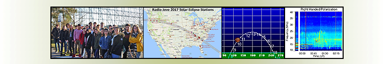
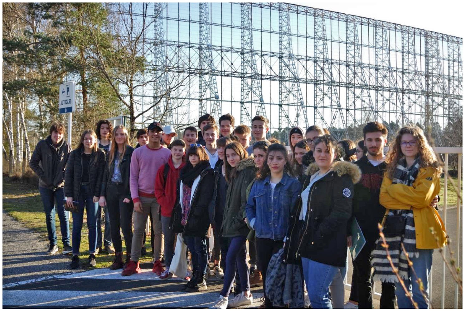
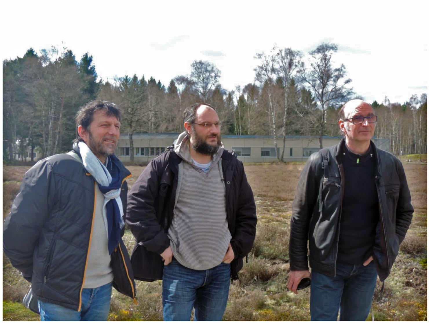
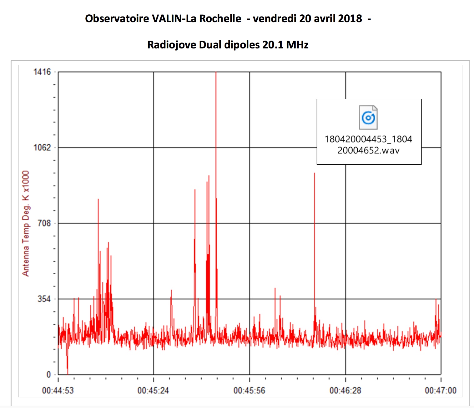
Denis Costa of the Lycée Valin in La Rochelle, France sent a report about recent successes with their Radio Jove observatory. As reported in the December 2016 Jove Bulletin, his students built a radio observatory on the campus of their school and were preparing for a trip to visit the Nancay Observatory. In 2018 April, Denis took a second group of students to Nancay and his observatory is now operational. He reports successful reception of solar radio bursts and a Jupiter Io-B radio storm. Congratulations!
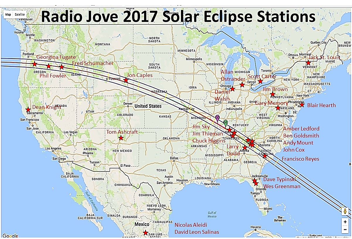
The Great American Eclipse of 2017 was a tremendous experience for those that got to witness it. First, we wish to thank the dedicated Radio Jove observers that took the time and made the effort to collect radio data during the eclipse. We had twenty-five successful persons/groups submit solar eclipse data to the Radio Jove archive. They are listed on the map in Figure 1. Again, thank you so much for your contributions to radio science!
This is a brief update on the progress of data analysis. We are comparing Radio Jove data from stations within the path of totality to those outside the path of totality to answer two questions: whether the presence of the Moon occulted the radio emitting regions near the Sun, and whether the Earth’s ionosphere was significantly affected by the umbral shadow of the Moon. The radio emission sources are located in the corona near the Sun and the solar eclipse radio measurements may help us to improve the accuracy of these source regions. Also, it is well known that the ionosphere changes significantly from daytime to nighttime and will affect the propagation of radio waves.
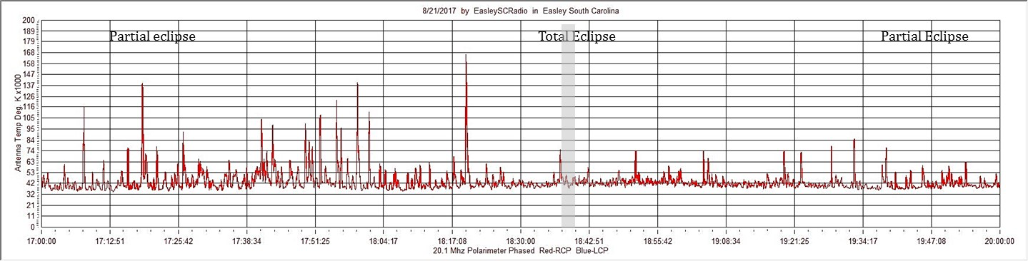
The Sun was very active on the day of the eclipse, and there was continuum bursting for many hours before, during, and after the eclipse. Many Radio Jove observers recorded these bursts, and an example from John Cox in Easley, SC is shown in Figure 2. The partial eclipse began just after 17:00 UT and ended about 20:00 UT with about 2.5 minutes of totality occurring at 18:37 UT. It appears that the number of bursts and the intensity of the bursts diminish after totality. However, the Sun is highly variable, the ionosphere is highly variable, and the observer’s local conditions are variable. Therefore, making quantitative comparisons is difficult.
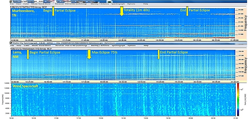
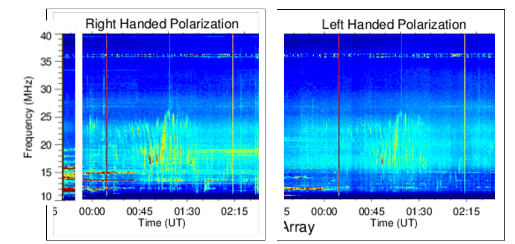
Another example, shown in Figure 3, is 15-30 MHz spectrograph data from me in Murfreesboro, TN and from Tom Ashcraft in Lamy, NM from 16:00 – 21:00 UT on August 21, 2017. We compare our ground-based data to the Wind spacecraft which is beyond the distance of the Moon and did not experience the eclipse. The Wind data in the bottom panel of Figure 3 show the continuous bursting of the Sun and give a baseline for solar variability. Initial analysis of these data show that the intensity of radio bursts are reduced near the time of totality in the Murfreesboro, TN data as compared with the data from Lamy, NM. However, as mentioned before, the variable nature of the data make for large errors, and thus it is difficult to draw quantifiable conclusions.
Again, thanks to your efforts and contributions to science we are making good progress. We hope to have more results in the near future.
Included with the Radio Jove kit are two very useful software packages for Windows PCs. The first, Radio Jupiter Pro, will help you plan when to make your Jupiter observations to increase the likelihood of success. The second, Radio Sky-Pipe enables you to record your data. Both of these software packages are from Radio-Sky Publishing.
In this article we will focus on an example of how Radio Jupiter Pro will help with planning for Jupiter observing; the specifics on configuring the software are available in the instruction manual.
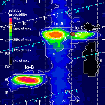
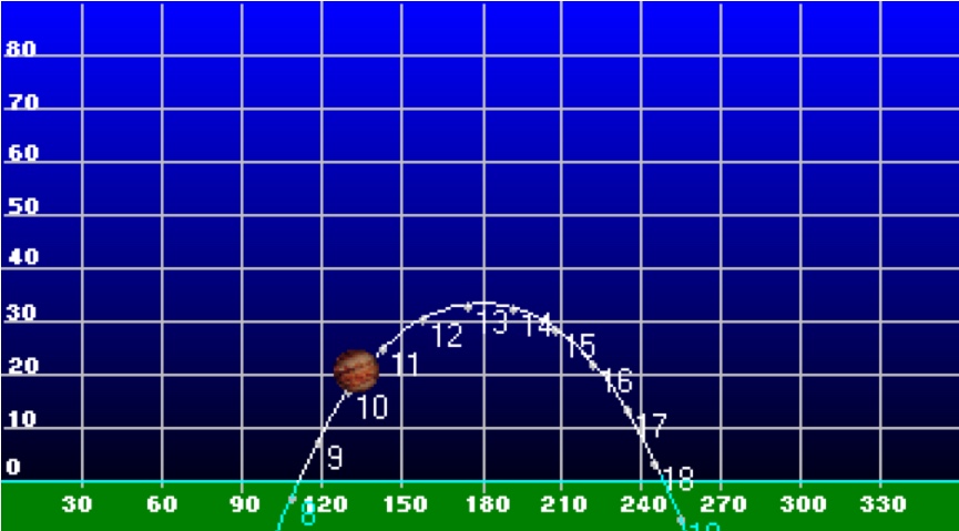
We will be using a real-life example from the observing run of Jim Brown. On 2018 January 6, as seen in Figure 1a (the CML-Io Phase plot), Jim noticed that there was a good opportunity to observe a Jupiter Io-C radio storm between the hours of 1000 and 1100 UT. He also noticed that Jupiter would be visible from his observatory in Pennsylvania, USA between approximately 0800 and 1800 UT. He found this by noting that the diagonal lines (indicating time) overlaid on the CML-Io Phase plot* crossed close to the center of the Io-C region between 1000 and 1100 UT. When these lines are white it indicates that Jupiter is above the horizon from your location, the blue lines mean that Jupiter is not visible. As shown in Figure 1b, during the predicted Io-C storm Jupiter appeared about 15 to 25 degrees above the horizon as seen from Jim's observatory. Jupiter will transit (that is it will reach its highest point in the sky) at about 1315 UT when it will be about 35 degrees above the horizon.
* For more details on the meaning of the CML (Central Meridian Longitude) - Io Phase plot please see the Radio Jove Science Brief on Jupiter’s Decametric Radio Emission and the June 2012 Jove Bulletin article for more on this topic.
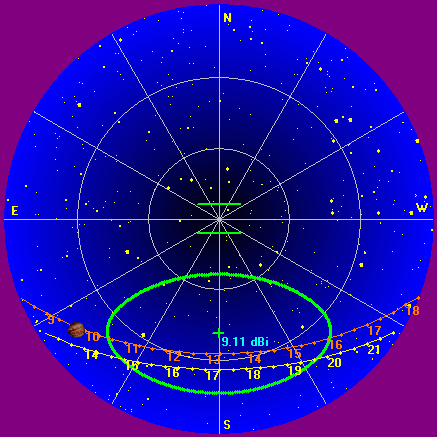
Jim Brown was using the Radio Jove dual dipole antennas aligned East-West. He added phasing cable between the dipoles to point the beam southward (see 2011 May Bulletin to read about phasing). In Figure 2 we see an illustration of the night sky with two green line segments representing his dipole array. The beam pattern (the region of sky where the antenna is sensitive) is the green oval towards the south. The times we want to observe are when Jupiter is within the beam. The beam is oriented such that the point of highest sensitivity (the green plus sign) is near the transit point of Jupiter (on this date that was at about 1315 UT). The figure also illustrates the paths that Jupiter and the Sun will be taking across the sky and the times at each location. Note that the Sun was not up at the time of the Io-C event. Jupiter observations should be made at night, because Earth's daytime ionopshere can make Jupiter radio observing much more challenging. We know from Figure 1a that we will be passing through Jupiter’s Io-C source between about 1000 and 1100 UT. At that time Jupiter was just moving into the antenna beam (crossing into the green ellipse). Even though the antenna was not at its most sensitive at this point, Jim was still optimistic about receiving Jupiter radio emissions.
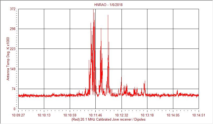
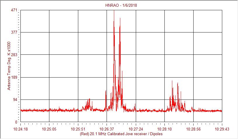
Figures 3 show us the Jupiter data recorded using Radio Sky-Pipe that Jim received between 1009 and 1029 UT on 2018 January 6. Of course there is no guarantee that you will detect Jupiter even when there is a predicted radio event occurring within your antenna beam; local weather conditions and local radio interference also may make it more difficult to successfully observe. As discussed in the May 2011 Jove Bulletin there are other factors that can influence observing Jupiter as well.
Imagining the Perfect Storm
Based on this example, can we now imagine what would have been the conditions for observing the "perfect storm"? First, we will want to be observing during a time period when we expect to pass through the heart of one of the Jupiter radio sources, namely the red or orange regions in Figure 1a. Second, Jupiter during this same time period should be nearly at transit from our location so that we will be able to detect these radio emissions even when they are weak. Third, these Jupiter radio observations should be made at night. Finally, our perfect storm observations should have great local conditions (no thunderstorms nor radio interference). You may not always have an opportunity to observe the perfect storm but don't let that prevent you from trying.
I hope this brief look at the Radio Jupiter Pro software will help you plan your next Jupiter observing run. Good luck!
After building the Radio Jove antenna and receiver, we want to record a radio signal at a fixed frequency of 20.1 MHz using the software Radio-SkyPipe II [1]. This software allows us to save this signal in the spd format. With a digital spectrometer, another software, Radio Spectrograph [2], can collect a radio spectrum in a wide band in the sps format. These files are publicly accessible through the Radio Jove data archive [3], thanks to individual amateur radio astronomers. Although the spd and sps data can be displayed in this software, they are only supported on Windows machines. In order to visualize and analyze the Radio Jove data on any operating system, we have produced these readers in Autoplot, which is a Java-based interactive browser [4]. Autoplot has been developed and maintained for the NASA Virtual Observatories for Heliophysics and is freely available. Autoplot has the capability of performing many powerful features including easy access to professional data (CDAWeb [5], Long Wavelength Array station One (LWA1) Jupiter data archive [6], and Nancay Decametric Array (NDA) database [7]), data analyses based on both Graphic User Interface (GUI) and scripting, and data communication with code written in IDL, MATLAB, and Python.
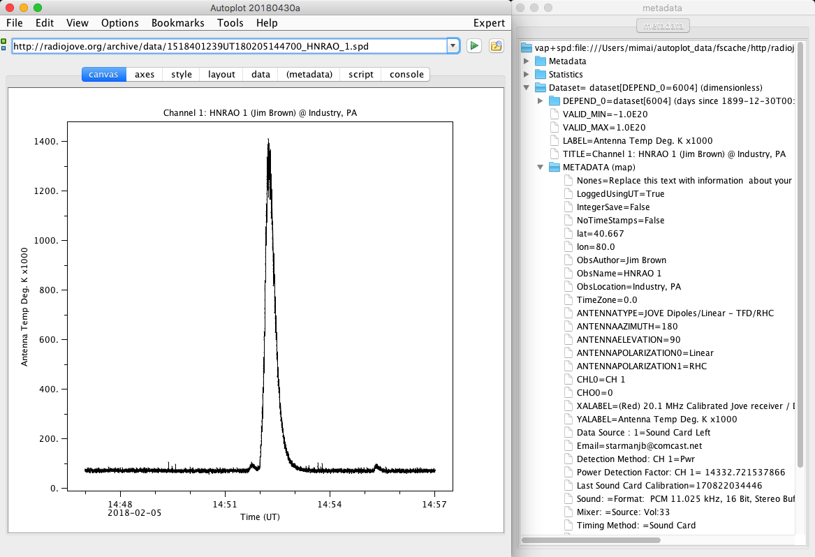
When opening Autoplot, you simply specify the locations of the Radio Jove data in the address bar. Simple, right? Let's see two examples for sps and spd files. Figure 1 shows an example Autoplot display of the Radio Jove spd data. The data include a nice Solar Type III burst event at 20.1 MHz on February 5, 2018. The data were collected at the Hawk's Nest Radio Astronomy Observatory (HNRAO) by Jim Brown. The right pane shows additional detailed information attached to this spd file.
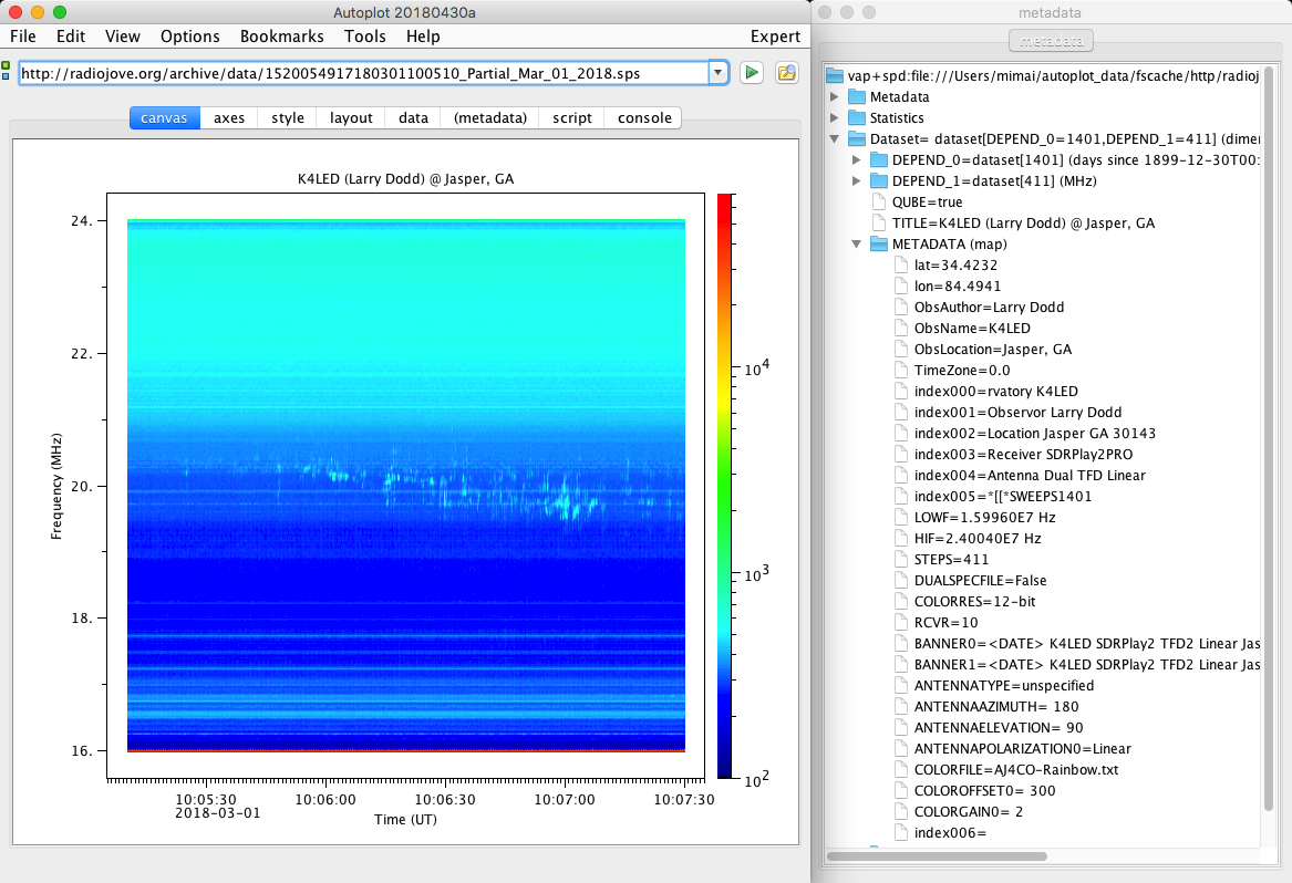
The second example, shown in Figure 2, is the Radio Jove sps data recorded at K4LED by Larry Dodd. This spectrogram covers a frequency range of 16 to 24 MHz, in which the strong Io-B Long-bursts were captured on March 1, 2018. Again, the right pane summarizes the supplemental information related to this observation.
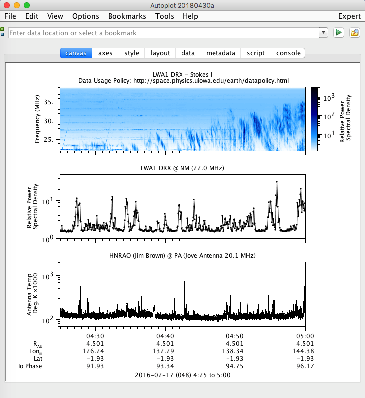
Taking advantage of Autoplot built-in features, we can easily compare the Radio Jove data with professional radio data, such as data from the LWA1 in New Mexico [8], at the same time. Figure 3 depicts (top) the LWA1 Jovian Io-B dynamic spectra, (middle) a 22.0-MHz LWA1 spectral density, and (bottom) a 20.1-MHz chart taken from the HNRAO's Jove antenna. The middle and bottom plots show similar variations, even with the 2-MHz frequency gap. Additionally, the LWA1 Jupiter project at the University of Iowa has provided Jovian ephemeris data from Earth. This ephemeris includes the distance between Earth and Jupiter in Astronomical Units (AU, RAU), System III west longitude (LonIII) and latitude (Lat), and Io phase. These are provided as additional values along the time axis at the bottom of the plot.
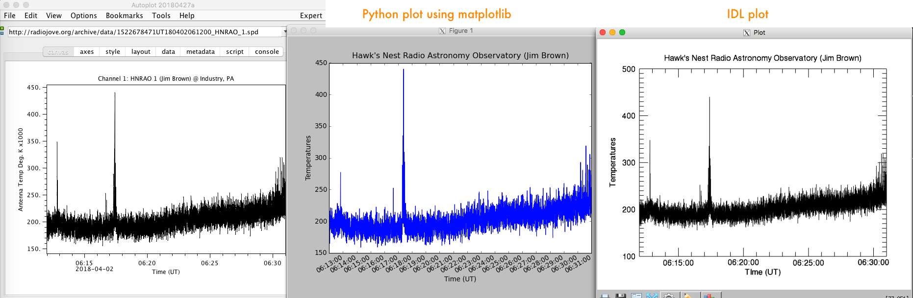
If you are intrigued by more data, why don't we perform scientific data reduction? One Autoplot feature is its ability to communicate with other languages, such as Python and IDL. Figure 4 shows a demonstration of retrieving the same Radio Jove spd file in Autoplot, Python, and IDL. Each language must be set up for the data communication with Autoplot. Some examples are available at: https://saturn.physics.uiowa.edu/svn/earth/public/radiojove/
A number of space projects in low-frequency radio astronomy have been carried out all over the world. One such project is NASA's Juno mission to Jupiter. Since the orbit insertion on July 4, 2016 (PDT), Juno has been listening to Jupiter's auroral radio sounds at a distance of ~100 Jovian radii, passing through the source of radio signals [9]. These data are accessible through the Planetary Data System. Meanwhile, the Juno-supporting ground-based Jupiter observation campaign is very active [10]. Because Jovian observation time from an Earth-based radio observatory is restricted to about 8 hours per day, the international coordination can continuously monitor Jovian auroral radio signals. We encourage amateur radio astronomers, participating in the NASA Radio Jove project, to coordinate their observations. After collecting data, we hope Autoplot will help you to unlock many Jovian radio mysteries.
We thank Jim Brown and Larry Dodd for the use of their Radio Jove data. We also appreciate the help from the engineers and staff who operate the LWA1 and support for the coordinated Juno-LWA1 Jupiter project, especially Greg Taylor.
References
The JOVE Bulletin is published twice a year. It is a free service of the Radio JOVE Project. We hope you will find it of value. Back issues are available on the Radio JOVE Project Web site, http://radiojove.gsfc.nasa.gov/
For assistance or information send inquiries to:
or
